Engineering: ANSYS/Forte
Overview
ANSYS Forte is the only CFD simulation package for internal combustion engines that incorporates proven ANSYS Chemkin-Pro solver technology – the gold standard for modeling and simulating gas phase and surface chemistry. Forte includes state-of-the-art automatic mesh generation (AMG), including solution adaptive mesh Refinement (SAM) and geometry-based adaptive mesh refinement (AMR). While legacy engine-combustion CFD simulations utilize chemistry solvers that are too slow to handle the chemistry details required for accurate predictions of ignition and emissions, Forte enables the use of multicomponent fuel models to combine with comprehensive spray dynamics – without sacrificing simulation time-to-solution.
Features
Automatic mesh generation that eliminates weeks of effort typically spent on manual mesh preparation
Embedded Chemkin-Pro solver technology that provides the computational speed required for predictive engine simulations
True multicomponent fuel-vaporization models that enable a self-consistent representation of the physical spray and the kinetics for accurate prediction of fuel effects
Advanced spray models that dramatically reduce grid and time-step dependency when compared to existing approaches
The ability to track soot particle nucleation, growth, agglomeration and oxidation without a compute-time penalty to predict particle size and number
Tutorial
This tutorial will describe the steps needed to complete the execution of the first examples from the tutorial documentation.
Connect to Mountaineer
ssh -X username@mountaineer.hpc.wvu.edu
The `-X` is necessary to get access to the graphical interface needed to prepare the simulation.
Load the Module
module load ansys/forte/17.2
Forte initial GUI
Execute the ANSYS/Forte GUI
First, we need to create a directory for the simulation we want to perform. Lets create for example a directory called ‘forte’ and inside create a subdirectory for our first simulation. The first simulation will be ‘SectorMesh’
mkdir $HOME/forte
mkdir $HOME/forte/SectorMesh
The Official Tutorials for Forte are in ‘/software/ansys_central/Forte_Tutorials’, we will copy Sandia_Engine_LTC_EarlyInj.ftsim to the directory we just create.
cp /software/ansys_central/Forte_Tutorials/Quick-start_SectorMesh/Sandia_Engine_LTC_EarlyInj.ftsim $HOME/forte/SectorMesh
We will use this input for this tutorial, now, we can launch the GUI using the command:
forte.sh &
The ‘&’ will free your terminal so you can enter more commands there. Otherwise you will need another terminal when we actually launch the simulation. Once you execute ‘forte.sh’ you should get a window with 3 buttons: Simulate, Monitor and Visualize.
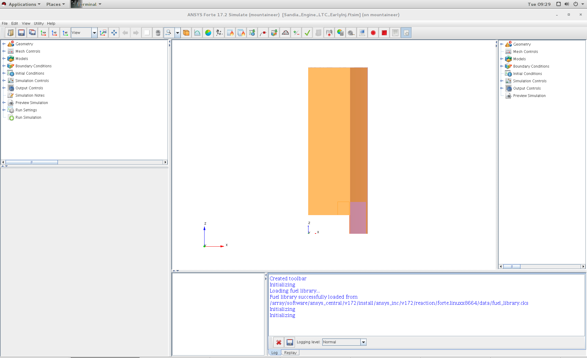
Simulate Window
Click on Simulate button and open the file `Sandia_Engine_LTC_EarlyInj.ftsim` You should get the ‘Simulate’ window. Click on Menu ‘File - Open…’ and search for the input file ‘Sandia_Engine_LTC_EarlyInj.ftsim’, in your directory ‘forte/SectorMesh’. The main window will display the mesh, you get on the log panel messages such
Loading fuel library...
Fuel library successfully loaded from
   /array/software/ansys_central/v172/install/ansys_inc/v172/reaction/forte.linuxx8664/data/fuel_library.cks
Initializing
Initializing
Now we are ready to create the scripts and run the simulation on Mountaineer
Simulate Window
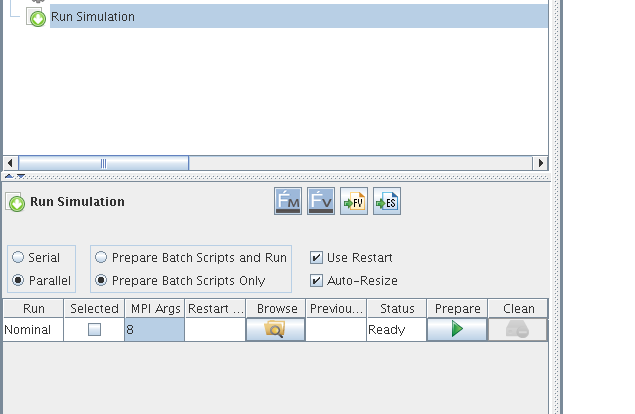
Prepare simulation files
Click on “Run Simulation” in the tree panel. The options for runnig the simulation appear in a panel down the tree panel. There are several options that we need to change. Select Parallel instead of Serial. Change to ‘Prepare Batch Scripts Only’. There is also a field under ‘MPI Args’, change that to the number of cores that you want use. 8 could be a reasonable number for this small simulation. Click the Green triangle under ‘Prepare’.
Now, we need to go back to the terminal and see the effects of preparing the simulation runs. A new directory is created called ‘Sandia_Engine_LTC_EarlyInj.analysis’. Inside that directory there are one file called ‘Sandia_Engine_LTC_EarlyInj.ftsim’ and a directory called ‘Nominal’ The contents of Nominal are:
chem.inp
chem.out
fuel_lib_chem.inp
fuel_lib_chem.out
fuel_lib_gas.asc
fuel_lib_xml.out
gas.asc
PREPARED
run_env.bat
run_env.sh
run_mpi.bat
run_mpi.sh
Sandia_Engine_LTC_EarlyInj.ftsim
therm.dat
xml.out
Now, we need to prepare the submission script for Mountaineer Go to ‘Nominal’ directory and create the script file
cd $HOME/forte/SectorMesh/Sandia_Engine_LTC_EarlyInj.analysis/Nominal
cat <<EOF >runjob.pbs
#!/bin/sh

#PBS -N FORTE
#PBS -l nodes=1:ppn=8,walltime=01:00:00
#PBS -m ae
##PBS -M username@mail.wvu.edu
#PBS -q hour

module load ansys/forte/17.2

cd $PBS_O_WORKDIR
sh run_mpi.sh
EOF
You should remove one # from ##PBS -M username@mail.wvu.edu and
change the email address in order to receive notifications when job
finish. We are requesting 1 hour (walltime=01:00:00), using one node
(nodes=1) and creating 8 MPI processes (ppn=8). Those values should be
adapted to the needs of your job. If you ask for more than one hour you
must change also the queue where you are submiting the jobs (#PBS -q
hour), consider for example queues ‘day’ and ‘week’ if your jobs need
more time to complete.
Submit the job with
qsub runjob.pbs
The job is submitted to the queue, it will start running when enough resources are free to start executing your job. You can always monitor the status of your submission with
qstat -u username
Once your job simulation start execution, you can monitor the progress by looking at the MONITOR file, one way of doing that is using tail command.
tail -f MONITOR
You should see something like
  7852    116.38  3.908E-02  5.000E-06  Maximum reached       953.80   330.53    0.4565  9.79E+00      15729       190
  7853    116.42  3.909E-02  5.000E-06  Maximum reached       953.70   330.51    0.4563  9.79E+00      15729       191
  7854    116.45  3.909E-02  5.000E-06  Maximum reached       953.60   330.49    0.4556  9.78E+00      15729       194
  7855    116.49  3.910E-02  5.000E-06  Maximum reached       953.50   330.48    0.4557  9.78E+00      15729       191
  7856    116.52  3.910E-02  5.000E-06  Maximum reached       953.41   330.46    0.4560  9.78E+00      15729       190
  7857    116.56  3.911E-02  5.000E-06  Maximum reached       953.31   330.44    0.4557  9.78E+00      15729       190
  7858    116.60  3.911E-02  5.000E-06  Maximum reached       953.21   330.42    0.4549  9.77E+00      15729       188
  7859    116.63  3.912E-02  5.000E-06  Maximum reached       953.12   330.41    0.4552  9.77E+00      15729       188

Cycle#   CA[deg]    Time[s]    Step[s]  Step constraint      MaxT[K]  MinT[K] MaxP[MPa] MaxV[m/s]     #Cells #Clusters
  7860    116.67  3.912E-02  5.000E-06  Maximum reached       953.02   330.38    0.4550  9.77E+00      15729       188
  7861    116.70  3.913E-02  5.000E-06  Maximum reached       952.92   330.37    0.4551  9.76E+00      15729       188
  7862    116.74  3.913E-02  5.000E-06  Maximum reached       952.82   330.35    0.4542  9.76E+00      15729       185
  7863    116.78  3.914E-02  5.000E-06  Maximum reached       952.72   330.33    0.4542  9.76E+00      15729       187
  7864    116.81  3.914E-02  5.000E-06  Maximum reached       952.63   330.32    0.4544  9.76E+00      15729       188
  7865    116.85  3.915E-02  5.000E-06  Maximum reached       952.53   330.29    0.4541  9.75E+00      15729       186
  7866    116.88  3.915E-02  5.000E-06  Maximum reached       952.43   330.28    0.4535  9.75E+00      15729       186
  7867    116.92  3.916E-02  5.000E-06  Maximum reached       952.33   330.26    0.4534  9.75E+00      15729       188
  7868    116.96  3.916E-02  5.000E-06  Maximum reached       952.23   330.25    0.4534  9.74E+00      15729       186
  7869    116.99  3.917E-02  5.000E-06  Maximum reached       952.13   330.23    0.4538  9.74E+00      15729       187

Cycle#   CA[deg]    Time[s]    Step[s]  Step constraint      MaxT[K]  MinT[K] MaxP[MPa] MaxV[m/s]     #Cells #Clusters
  7870    117.03  3.917E-02  5.000E-06  Maximum reached       952.03   330.21    0.4535  9.74E+00      15729       189
  7871    117.06  3.918E-02  5.000E-06  Maximum reached       951.93   330.19    0.4527  9.74E+00      15729       192
  7872    117.10  3.918E-02  5.000E-06  Maximum reached       951.83   330.18    0.4528  9.73E+00      15729       192
  7873    117.14  3.919E-02  5.000E-06  Maximum reached       951.73   330.16    0.4530  9.73E+00      15729       192
The screen will update when the execution advances. When simulation finishes you should get a summary of execution like
============================================================
Engine Summary Data:
------------------------------------------------------------
Cylinder Index 1
------------------------------------------------------------
Power 9.84048 [kW]
IMEP 0.42126 [MPa]
Fuel Mass 5.35000E-002 [g/cyc]
Fuel Lower Heating Value 44.52000 [kJ/g]
Gross ISFC 195.72213 [g/kW-h]
ISFC(IVC->EVO) 223.19199 [g/kW-h]
Total Chemical Heat Release 2376.63829 [J]
Total Heat Release From P-V 1297.21755 [J]
Combustion Efficiency 0.99782 []
Thermal Efficiency 0.41315 []
Max Pressure 8.62842 [MPa]
Max Temperature 1262.21947 [K]
Max Pressure Rise Rate 0.84582 [MPa/deg]
CA @ 2% Heat Release -14.97600 [deg ATDC]
CA @ 10% Heat Release -8.99000 [deg ATDC]
CA @ 30% Heat Release -5.98561 [deg ATDC]
CA @ 50% Heat Release -5.98561 [deg ATDC]
CA @ 90% Heat Release 0.02813 [deg ATDC]
10%-90% Heat Release Duration 9.01813 [deg]
Soot @ EVO 3.66015E-004 [g/kg-f]
7.16372E-005 [g/kW-h]
8.72851E-006 [ppm]
EINOx @ EVO 3.39138E+000 [g/kg-f]
6.63767E-001 [g/kW-h]
2.09039E+001 [ppm]
CO @ EVO 2.17074E+001 [g/kg-f]
4.24862E+000 [g/kW-h]
2.19759E+002 [ppm]
UHC @ EVO 1.30878E+001 [g/kg-f]
2.56157E+000 [g/kW-h]
C1-UHC @ EVO 2.59096E+002 [ppm]
VOC @ EVO 1.35866E+001 [g/kg-f]
2.65920E+000 [g/kW-h]
C1-VOC @ EVO 2.63832E+002 [ppm]
============================================================
Normal termination: Cycle# 8092, CrankAngle[deg] 125.00, Time[s] 4.0278E-02
CGNS solution file closed successfully
================================================================================
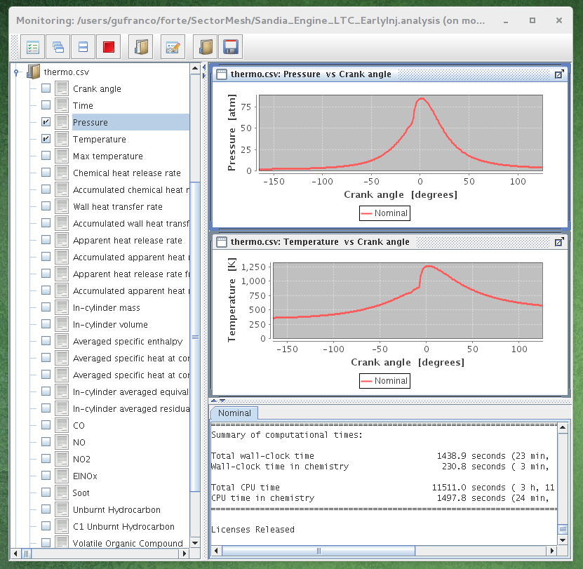
Summary of computational times:
Total wall-clock time 1438.9 seconds (23 min, 58.9 sec)
Wall-clock time in chemistry 230.8 seconds ( 3 min, 50.8 sec)
Total CPU time 11511.0 seconds ( 3 h, 11 min, 51.0 sec)
CPU time in chemistry 1497.8 seconds (24 min, 57.8 sec)
================================================================================
Licenses Released
Many files are now on you Nominal directory.
chem_0      chemsolver.csv        fuel_library_diag_0  gas.asc
chem_0.out  COMPLETE              fuel_library_diag_1  massfraction.csv
chem_1      dynamic.csv           fuel_library_diag_2  memory_diagnostics.csv
chem_1.out  flow_diagnostics.csv  fuel_library_diag_3  molefraction.csv
chem_2      FORTE.e107840         fuel_library_diag_4  MONITOR
chem_2.out  FORTE.log             fuel_library_diag_5  nc14h30_fueltable.csv
chem_3      FORTE.o107840         fuel_library_diag_6  Nominal_CA_p_125.00_8092.ftrst
chem_3.out  fuelchem_0            fuel_library_diag_7  Nominal.ftavg
chem_4      fuelchem_0.out        fuel_lib_xml.out     Nominal.ftind
chem_4.out  fuelchem_1            fueltable.out        Nominal.ftres
chem_5      fuelchem_1.out        fueltran_0           run_env.bat
chem_5.out  fuelchem_2            fueltran_0.out       run_env.sh
chem_6      fuelchem_2.out        fueltran_1           runjob.pbs
chem_6.out  fuelchem_3            fueltran_1.out       runjob.pbs~
chem_7      fuelchem_3.out        fueltran_2           run_mpi.bat
chem_7.out  fuelchem_4            fueltran_2.out       run_mpi.sh
chemdiag_0  fuelchem_4.out        fueltran_3           Sandia_Engine_LTC_EarlyInj.ftsim
chemdiag_1  fuelchem_5            fueltran_3.out       speciesmass.csv
chemdiag_2  fuelchem_5.out        fueltran_4           spray.csv
chemdiag_3  fuelchem_6            fueltran_4.out       therm.dat
chemdiag_4  fuelchem_6.out        fueltran_5           thermo.csv
chemdiag_5  fuelchem_7            fueltran_5.out       wall_heat_transfer.csv
chemdiag_6  fuelchem_7.out        fueltran_6           whole_domain_parameters.csv
chemdiag_7  fuel_lib_chem.inp     fueltran_6.out       xml.out
chem.inp    fuel_lib_chem.out     fueltran_7
chem.out    fuel_lib_gas.asc      fueltran_7.out
The best way of continue from here is to copy those files back to your workstation for post-processing and analysis.
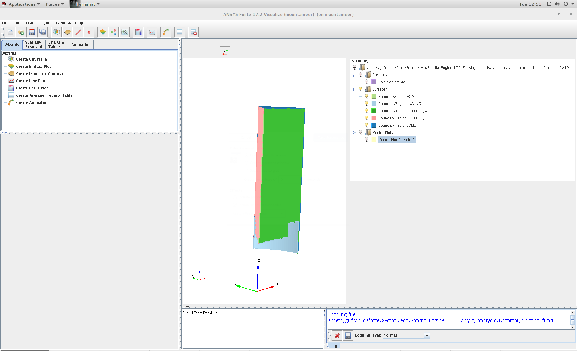
You can however continue on Mountaineer and start analysing the results of the simulation. On the initial window with three buttons, click on Monitor and open the project file. The image on the left, you can get see basic plots of temperature and pressure as a function of crank angle. By clicking on the Visualize button you get a big window where you can see visualizations of the fluids inside the crank.
asdsadsd