Web Interface (Open On-Demand)
The term Interactive Scientific Computing consists of using a computer in a similar way as you use a handheld calculator. On a handheld calculator, you type some input and you expect that input to be processed right away to produce results. The result does not need to return immediately, but you expect that calculations that are done take an amount of time that allows a human to wait before a new command is submitted.
Interactive Scientific Computing is different from the way we use to work in High-Performance Computing (HPC). On an HPC supercomputer, you use the computer with a queue system on what we called non-interactive computing. Supercomputers are large computing devices usually build as clusters of individual computers. Supercomputers in many cases are used by tens or hundreds of users at the same time. For the typical use of Supercomputers, the computations are programmed in advance, the user submits jobs expecting that those jobs start being executed sometime in the future and produce the result that will be analyzed later on.
Despite the usual usage of HPC supercomputing, you could have strong motivations for using a computer far more powerful than your own desktop or laptop. Your research has scaled to a point where your desktop computer or laptop is no longer capable of managing the task, you need specialized software packages and you do not want to spend time compiling or installing software and you would like to rely on software that is already present on the HPC cluster.
There are several ways to a HPC cluster for Interactive Computing. You can execute interactive computing directly from the terminal or using a web interfact such as Open-On Demand and one interactive environments such as Jupyter of RStudio. We will describe both alternatives.
Interactive Computing from the Terminal
First, connect to the cluster using the instructions described on here:ref:qs-connect:. Once on the head node you can request an interactive session with:
trcis001:~$ module load sched/slurm/22.05
trcis001:~$ srun --pty bash
This is the simplest command for requesting an interactive session. Under this command, the partition selected will be standby with a walltime of 4 hours.
The job will be allocated on one compute node and one core on that node for the execution.
You can request more cores for your interactive job, for example:
trcis001:~$ srun -n 4 --pty bash
On Spruce Knob you can request 16 cores for an entire node. There are a few nodes with 20 and 24 cores but requesting with those numbers will reduce the chances of getting a node for your execution inmeately. On Thorny Flat most nodes have 40 cores. In contrast, Dolly Sods nodes focus on their GPU card. A way of requesting an entire node could be:
$> qsub -I -n
Requesting more than 1 core does not necessarily means that your code will actually using those extra cores. It all depends on your code being able to work in parallel directly or indirectly. Directly means that the code use some sort of paralelization such as multithreading such as pthreads or OpenMP, or multiprocessing such as MPI, or any other paralleization in languages such as R or Python that offer libraries for explicit parallelism. Indirectly paralleization means that underlying libraries such as FFTW or OpenBLAS could have been compiled with multithreading support meaning that codes that uses those libraries could take indirectly advantage of parallelism.
You can also request GPUs for an interactive job, in that case you have to explicitly request a queue such as comm_gpu_inter that offers compute nodes with GPU cards and explicitly request the number of GPUs that you want to use. For example if you want to use one GPU card for your execution use:
trcis001:~$ srun --pty -p comm_gpu_inter -N 1 -n 8 -G 1 bash
After you submit your request for interactive jobs, you will have to wait a few minutes before you are assigned a compute node. After getting access to the compute node, you can load modules and execute commands as you were on a machine. There are several text-based environments for interactive computing.
One is R and you can access it with:
$> module load lang/r/4.2.0_gcc112
$> R

R version 4.2.0 (2022-04-22) -- "Vigorous Calisthenics"
Copyright (C) 2022 The R Foundation for Statistical Computing
Platform: x86_64-pc-linux-gnu (64-bit)

R is free software and comes with ABSOLUTELY NO WARRANTY.
You are welcome to redistribute it under certain conditions.
Type 'license()' or 'licence()' for distribution details.

Natural language support but running in an English locale

R is a collaborative project with many contributors.
Type 'contributors()' for more information and
'citation()' on how to cite R or R packages in publications.

Type 'demo()' for some demos, 'help()' for on-line help, or
'help.start()' for an HTML browser interface to help.
Type 'q()' to quit R.

> sessionInfo()
R version 4.2.0 (2022-04-22)
Platform: x86_64-pc-linux-gnu (64-bit)
Running under: Red Hat Enterprise Linux Server 7.9 (Maipo)

Matrix products: default
BLAS/LAPACK: /gpfs20/shared/software/libs/openblas/0.3.19_gcc112/lib/libopenblas_skylakexp-r0.3.19.so

locale:
 [1] LC_CTYPE=en_US.UTF-8       LC_NUMERIC=C
 [3] LC_TIME=en_US.UTF-8        LC_COLLATE=en_US.UTF-8
 [5] LC_MONETARY=en_US.UTF-8    LC_MESSAGES=en_US.UTF-8
 [7] LC_PAPER=en_US.UTF-8       LC_NAME=C
 [9] LC_ADDRESS=C               LC_TELEPHONE=C
[11] LC_MEASUREMENT=en_US.UTF-8 LC_IDENTIFICATION=C

attached base packages:
[1] stats     graphics  grDevices utils     datasets  methods   base

loaded via a namespace (and not attached):
[1] compiler_4.2.0
>
Another text-based interactive environment is IPython, to use it execute for example:
$> module load lang/python/cpython_3.10.1_gcc112
Loading gcc version 11.2.0 : lang/gcc/11.2.0
Loading python version cpython_3.10.1_gcc112 : lang/python/cpython_3.10.1_gcc112

$> ipython
Python 3.10.1 (main, Dec 28 2021, 19:48:41) [GCC 11.2.0]
Type 'copyright', 'credits' or 'license' for more information
IPython 7.30.1 -- An enhanced Interactive Python. Type '?' for help.

In [1]: import platform

In [2]: platform.machine()
Out[2]: 'x86_64'

In [3]: platform.version()
Out[3]: '#1 SMP Thu Mar 25 21:21:56 UTC 2021'

In [4]: platform.platform()
Out[4]: 'Linux-3.10.0-1160.24.1.el7.x86_64-x86_64-with-glibc2.17'

In [5]: platform.uname()
Out[5]: uname_result(system='Linux', node='trcis001.hpc.wvu.edu', release='3.10.0-1160.24.1.el7.x86_64', version='#1 SMP Thu Mar 25 21:21:56 UTC 2021', machine='x86_64')

In [6]: platform.system()
Out[6]: 'Linux'

In [7]: platform.processor()
Out[7]: 'x86_64'
Matlab is another software that offers interactive environment. Usually MATLAB is accessed on a graphical interface but MATLAB can also work from a text-based interface:
$> module load lang/gcc/9.3.0 matlab/2021a
Loading gcc version 9.3.0 : lang/gcc/9.3.0

$> matlab -nodesktop
MATLAB is selecting SOFTWARE OPENGL rendering.

                                                                                                                                         < M A T L A B (R) >
                                                                                                                   Copyright 1984-2021 The MathWorks, Inc.
                                                                                                                   R2021a (9.10.0.1602886) 64-bit (glnxa64)
                                                                                                                                          February 17, 2021


To get started, type doc.
For product information, visit www.mathworks.com.

>>
Interactive Computing from a web interface
For taking advantage of WVU’s High Performance Computing cluster for interactive scientific computing another alternative is from a web browser. On this lesson you will not have to learn Linux commands, you just need to execute one for the purpose of downloading all the materials for the tutorials but beyond that your interaction will take place on a friendly web interface. You do not have to manually submitting jobs or editing submission scripts, these are tasks very important for HPC but they will delegated for other lesson.
We will be using a tool, a web-based client portal, that hides all that complexity and allow you to start using powerful computers for your research from a web interface, with minimal effort and fast learning curve.
Several technologies are involved here and it is important to understand how those different pieces are interconnected.
Open OnDemand is a web-based client, based on the Ohio Supercomputer Center’s proven “OSC On Demand” platform, that enables HPC centers to install and deploy advanced web and graphical interfaces for their users. HPC resources are accessible from a web browser without the user having to install any special software or plugin.
The path for this tutorial is as follows. First we will demonstrate how to access the open on demand portal. Next we will create Jupyter and RStudio sessions and opening a terminal and a file manager.
Accessing the Dashboard
First, go to Thorny Flat On Demand Dashboard or Dolly Sods On Demand Dashboard.
The first page you will see is asking for your credentials

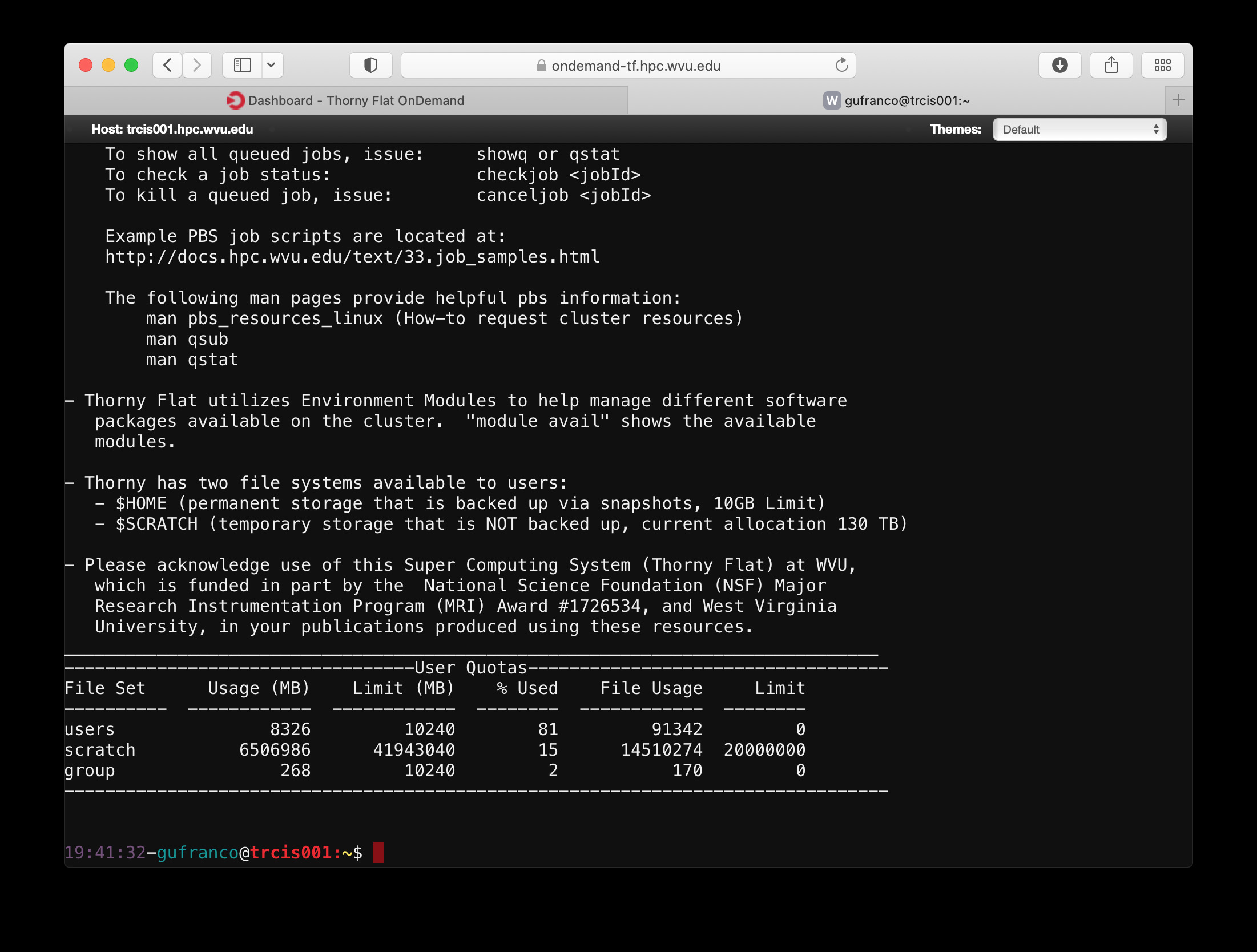
After entering your credentials and using your DUO authentication you will land on the Open On Demand Dashboard:
From this dashboard you can launch interactive jobs, open terminals and access a file manager, we will see each of those operations in the next sections.
Interactive applications
From the dashboard go to Interactive Apps. There are several options there, we will show 2 apps that are currently ready for being used. Jupyter Notebooks and RStudio.
Jupyter
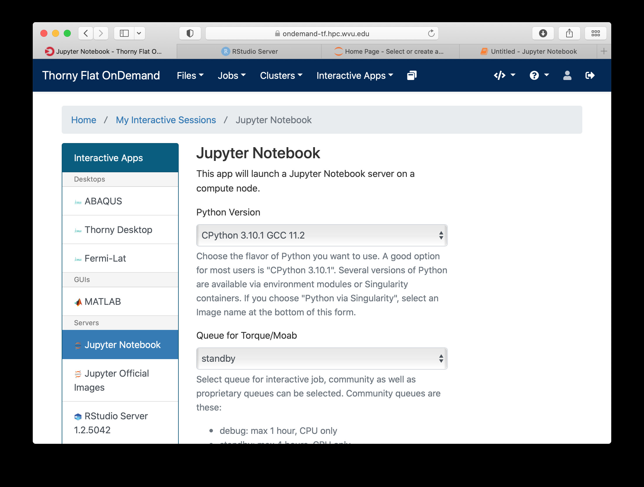
For Jupyter click on Ìnteractive Apps > Jupyter Notebook. A form is shown with all the options available to create the Jupyter session.
A good starting point is to select CPython 3.7.4 as the Python version, select standby as the queue and 4 hours as the wall time. There are options for alternative Python versions, queues and walltimes. A short description of each options is shown on the form.
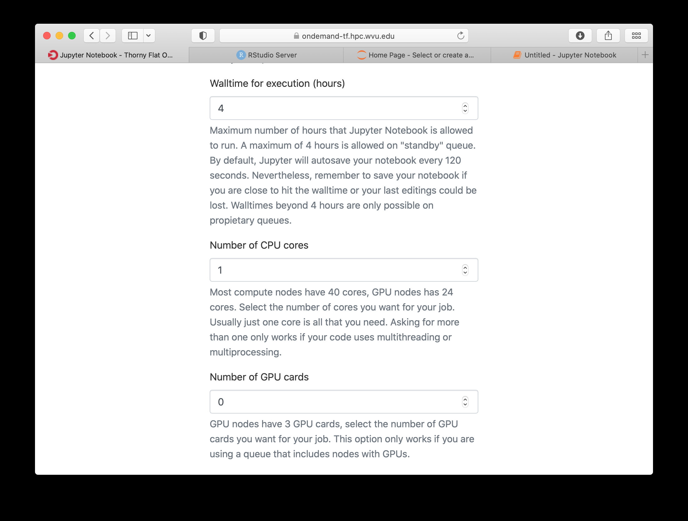
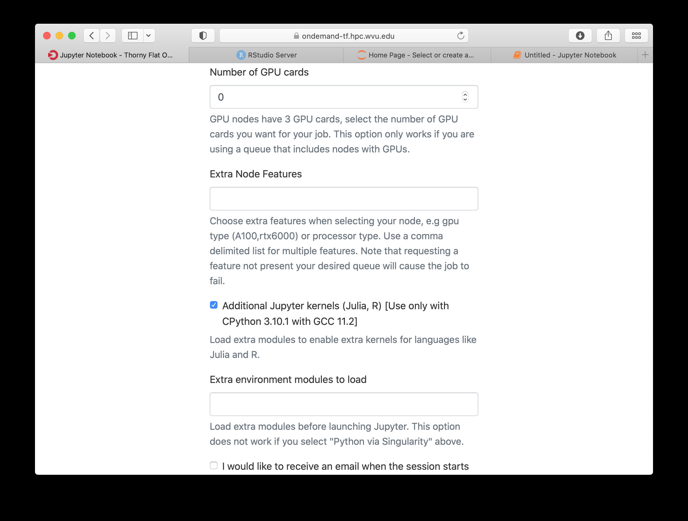
The next fields on the form ask for the number of cores, GPU cards, extra modules and the singularity image in case you have selected that as your Python version.
Notice that taking advantage of multiple cores depends on your code being able to use those cores. In the case of Python that usually means that your code is using multiprocessing module or you are using numpy with multi-threading capabilities. The usage of multiple cores is not something that happens automatically so if you are not sure asking for one core is enough. A similar situation happens with GPUs noticing that only the queue comm_gpu_inter give you access to GPUs for community nodes.
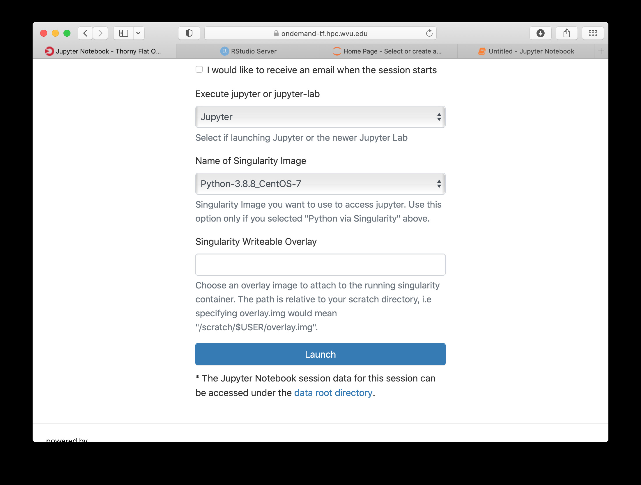
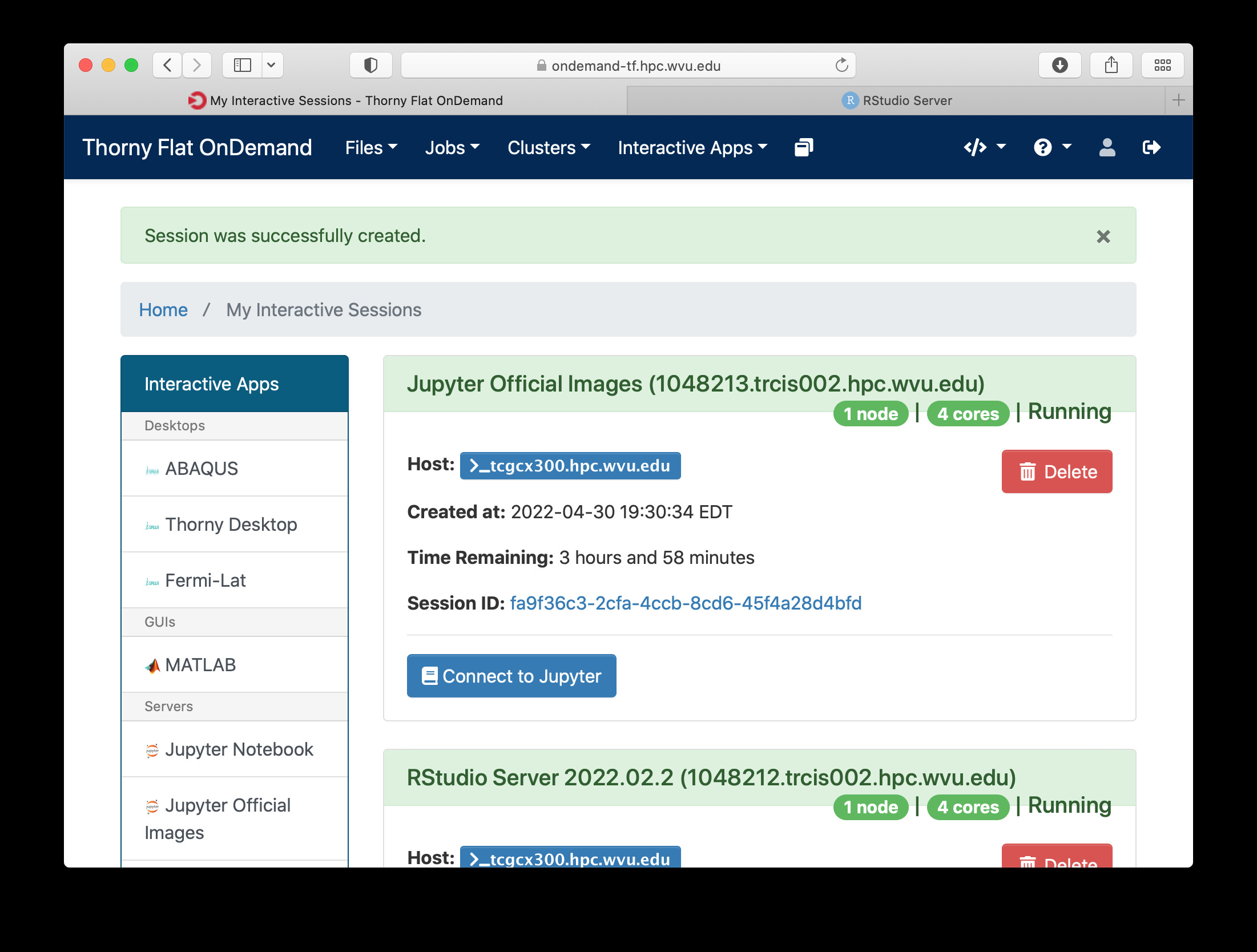
Once you have customize the parameters for your Jupyter session, click on Launch. Open On demand will launch a new interactive session and when the interactive session is launched you will get a button to connect to the Jupyter notebook.
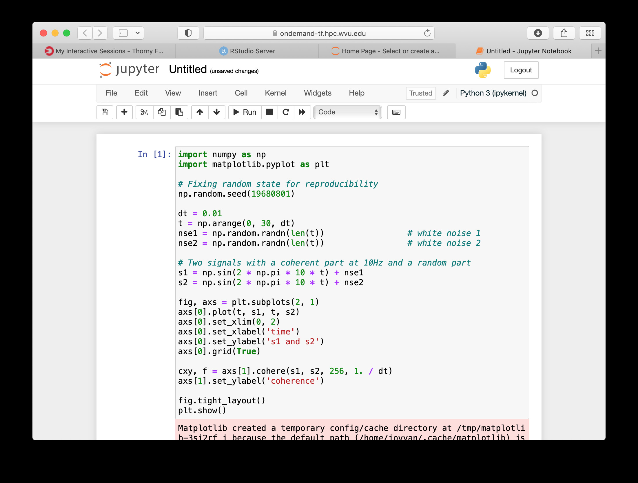
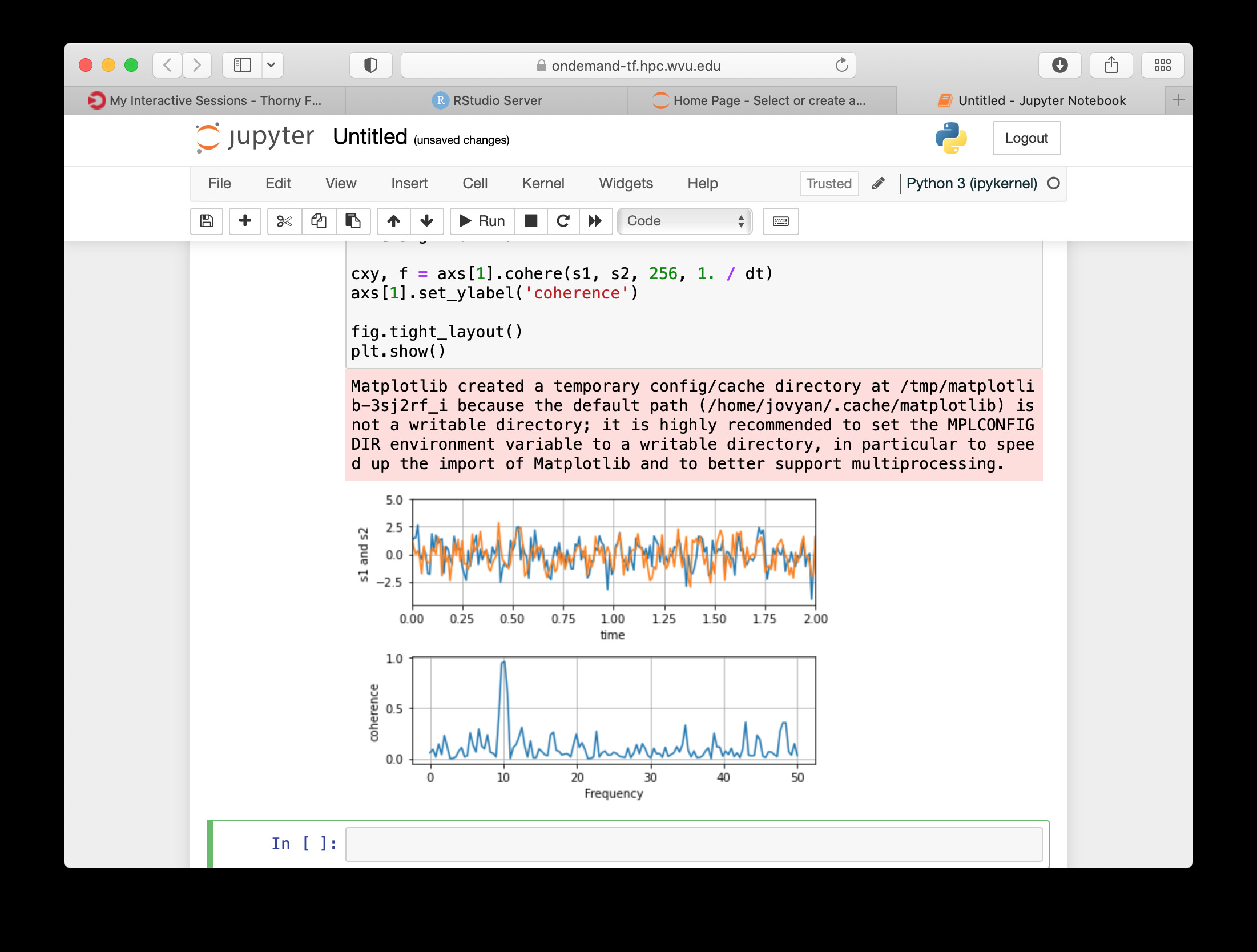
The Jupyter session is launched on a compute node. The Jupyter interface shows as file manager where you can select a notebook to launch, upload one from your local computer or create a new Notebook, go to New > Python 3 to create a new Jupyter notebook with Python 3 as kernel.
The new notebook give you entries for typing Python instructions that are executed when you type SHIFT-ENTER
RStudio
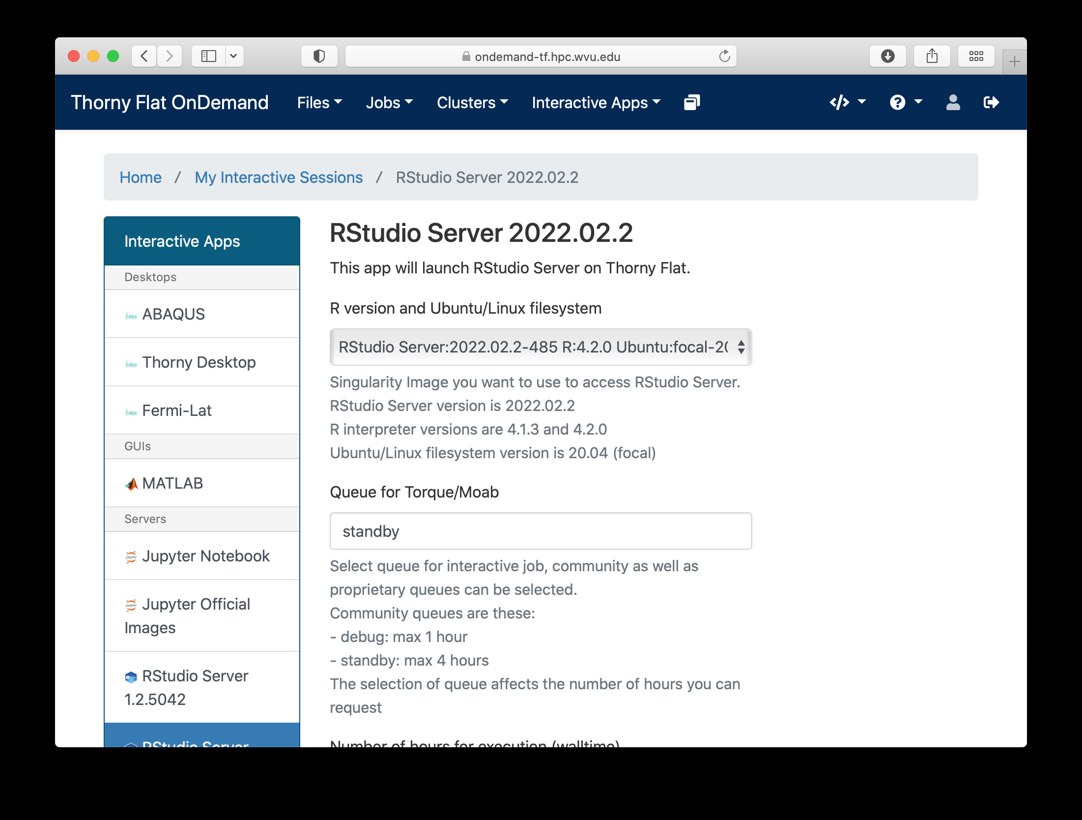
Another popular interactive environment is RStudio, select Interactive Apps > RStudio. The options in the form are very few. Select a queue such as standby, 4 hours of wall time and 1 core.
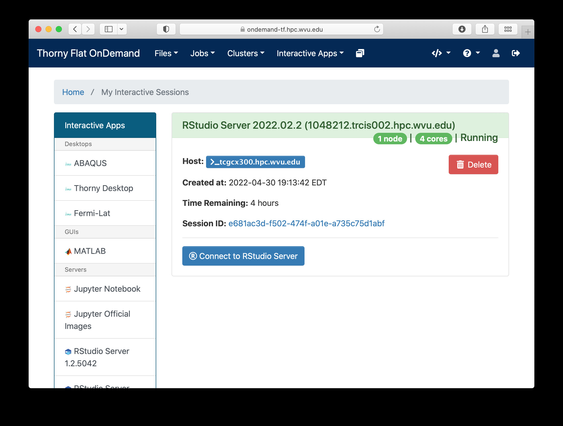
When you click on Launch, Open on Demand will create a new interactive session on Thorny Flat and when the job starts execution, a button appears to open the session on a new tab.
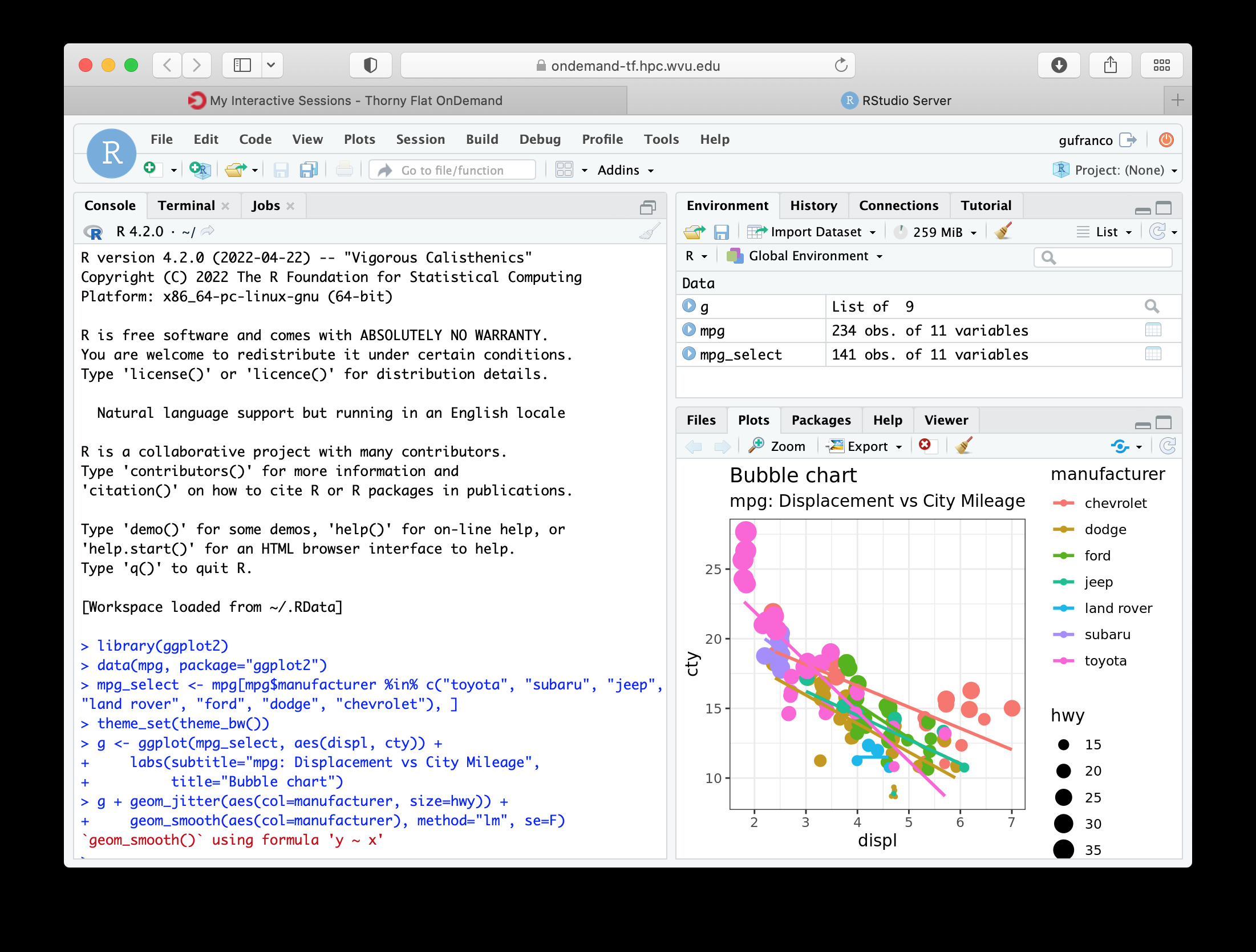
The interface for RStudio shows the commands on the left and variables and plots on the right.
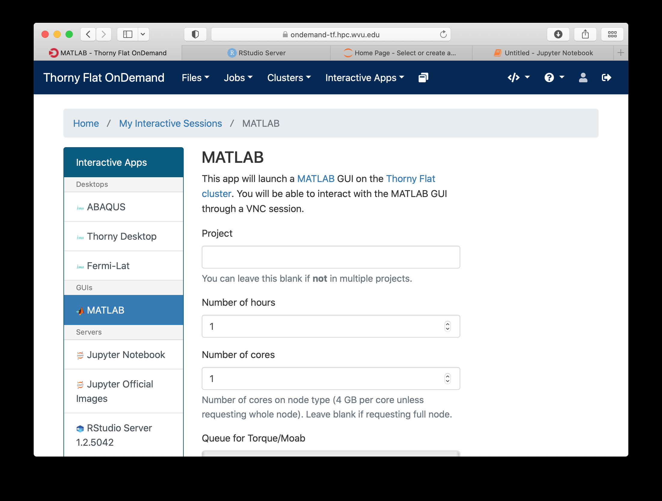
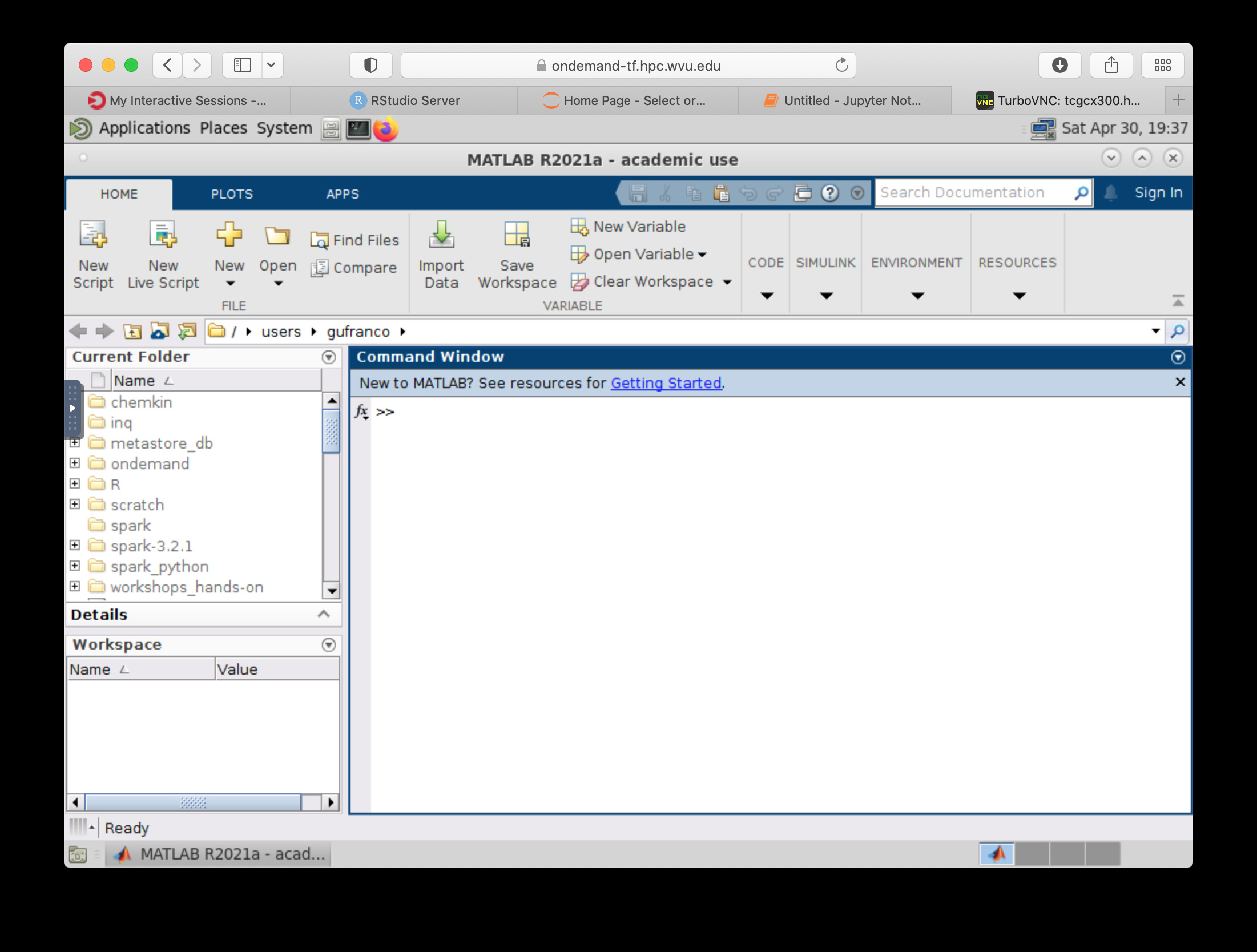
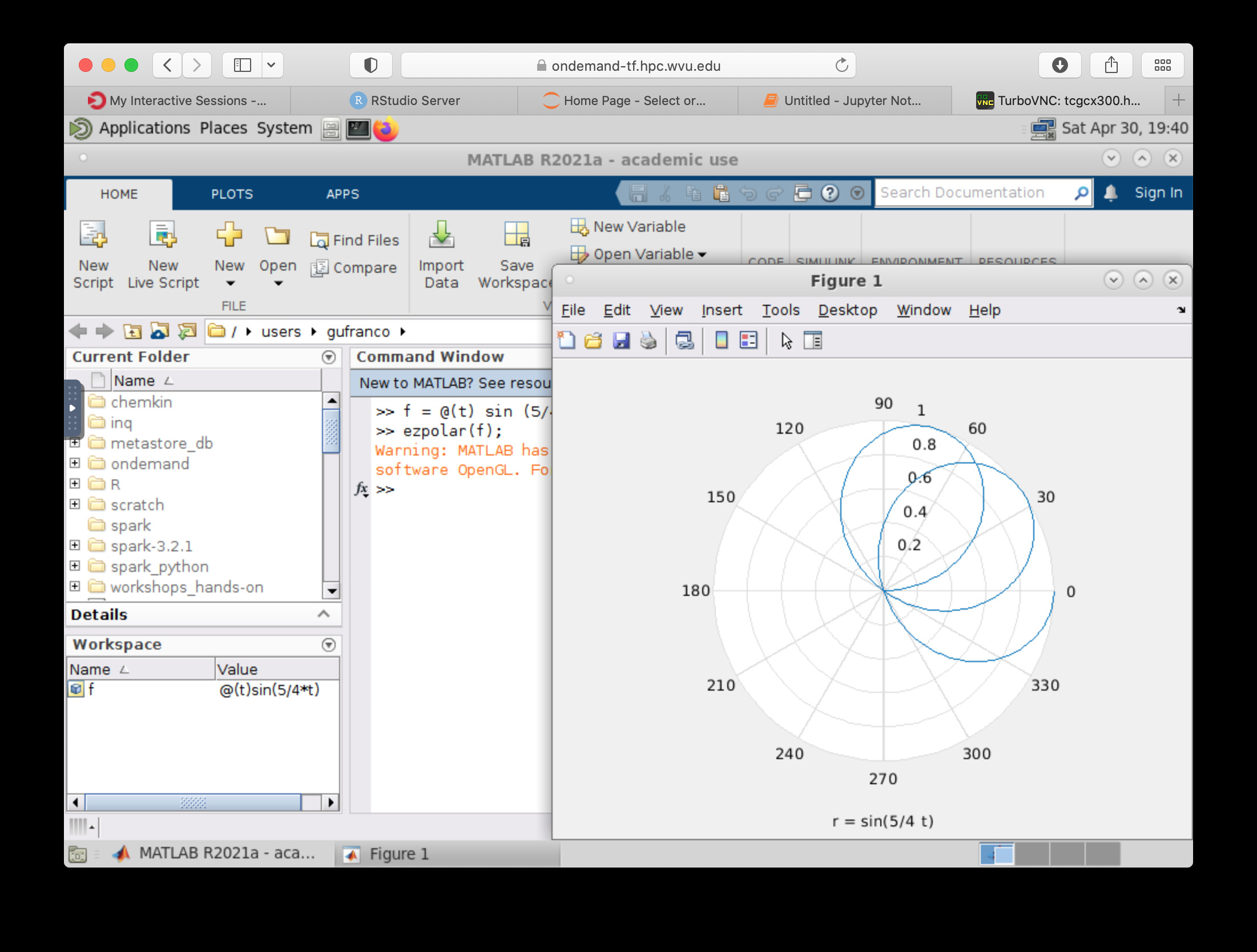
MATLAB
MATLAB is a numeric computing environment and programming language developed by MathWorks. MATLAB allows matrix manipulations, plotting of functions and data, implementation of algorithms, creation of user interfaces, and interfacing with programs written in other languages. MATLAB can run using Open On-Demand via an app that executes a virtual desktop on a browser tab.
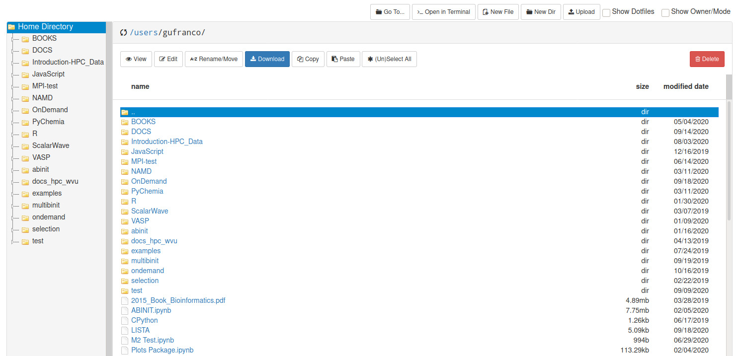
File Manager
The Open On demand dashboard also offers a simple but useful File Manager that give you options to view, edit, download and rename files. It is a simple way to see plots and download individual files to your local computer.
To access the File Manager on the Dashboard, go to Files > Home Directory. The File Manager is shown as
Job manager
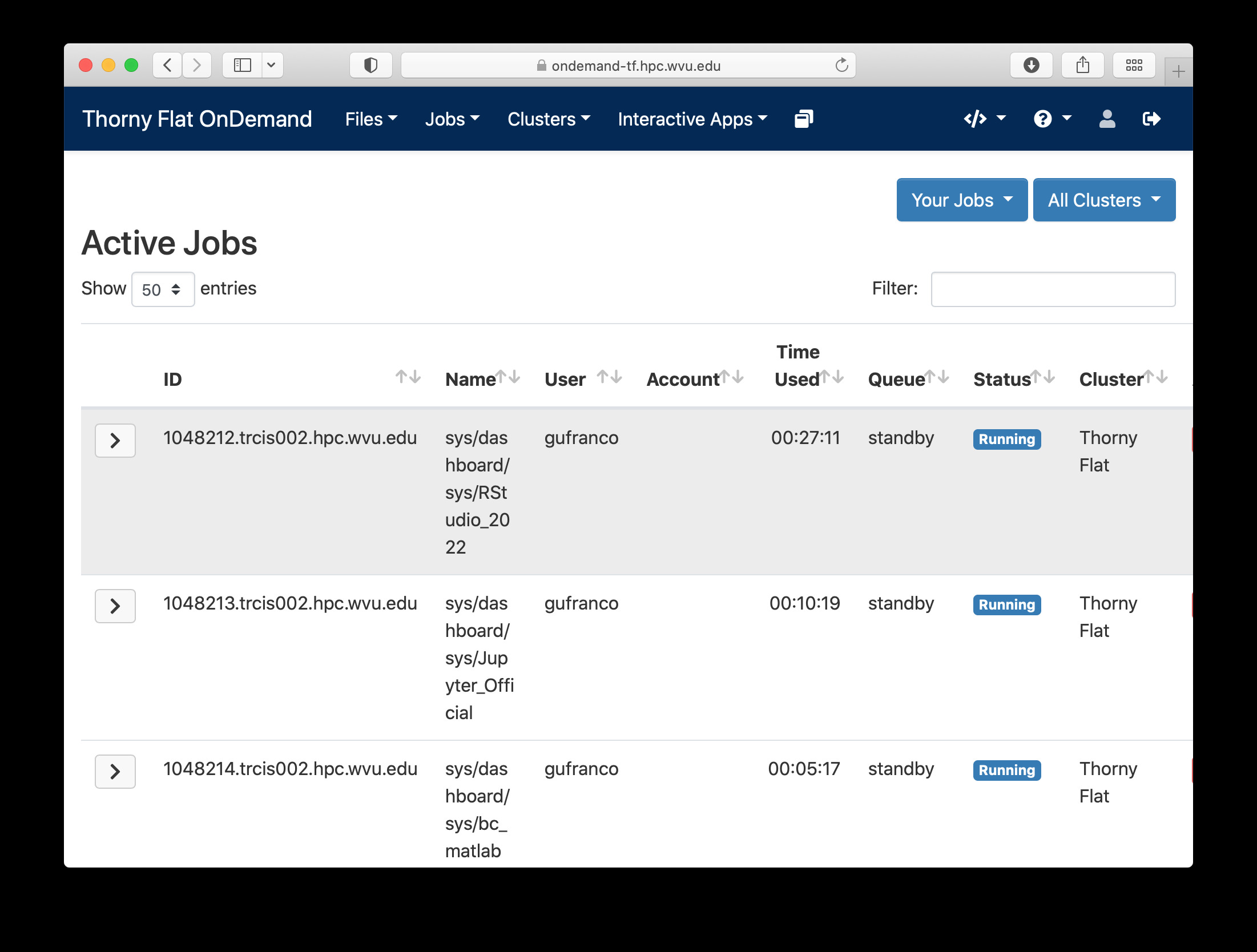
Another useful tool integrated with the Dashboard is the Job Manager, you can see the jobs currently submitted on the cluster. Go to Jobs > Active Jobs to access the Job Manager
Job composer
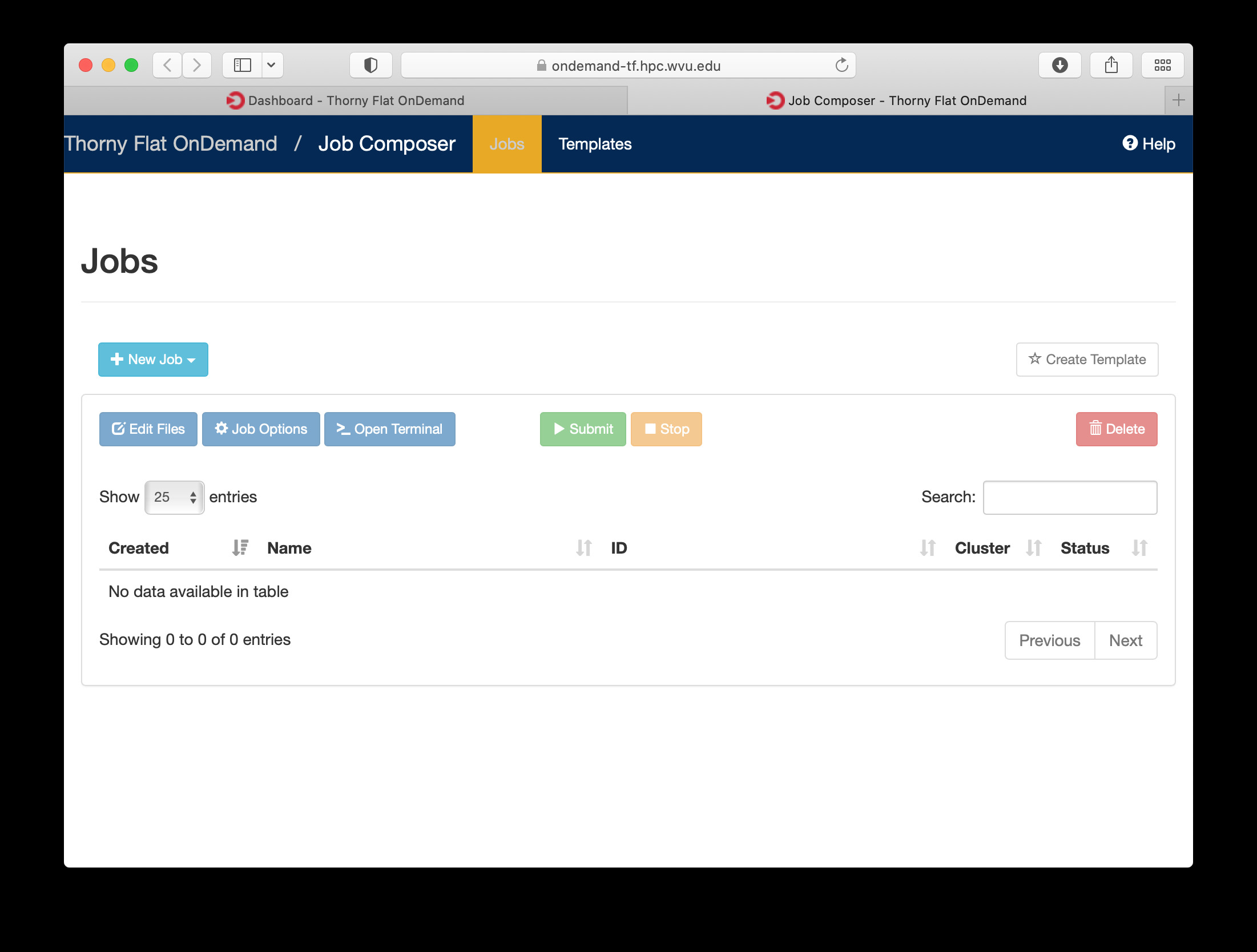
Another useful tool integrated with the Dashboard is the Job Composer, you can create jobs and submit them to the cluster via a web interface. Go to Jobs > Jobs Composer to access the tool.
Terminal
Finally a Terminal session can be opened from the dashboard, the terminal runs on the head node exactly as a normal connection to the cluster via SSH. It has, however a short limit of time to be alive if no command is typed on it. The terminal is intended for quick commands only.